How to make summary tables in Excel

When working with spreadsheets in Office Excel, it is often necessary to organize a large number of rows into visual reports. This is easy enough to do if you follow these simple instructions.

What is a summary table in Excel and what is it for?

A summary table is a special tool for detailed data analysis in Excel. It collects various information from standard tables, performs processing, categorization and a number of calculations for further publication of the result in the form of reports. And all report parameters can be customized to meet your requirements.

Summary tables are indispensable when you need to prepare a detailed report from a large number of different data. They summarize randomly placed values and then group them in a convenient format for advanced calculations.
The layout of the summary table is easy to customize to your preferences with a couple of mouse clicks. For example, you can change column and row locations, filter totals, and move report blocks from one point to another for greater clarity.
Let’s look at the intricacies of working with summary tables using a practical example.

Step 1: Creating a table

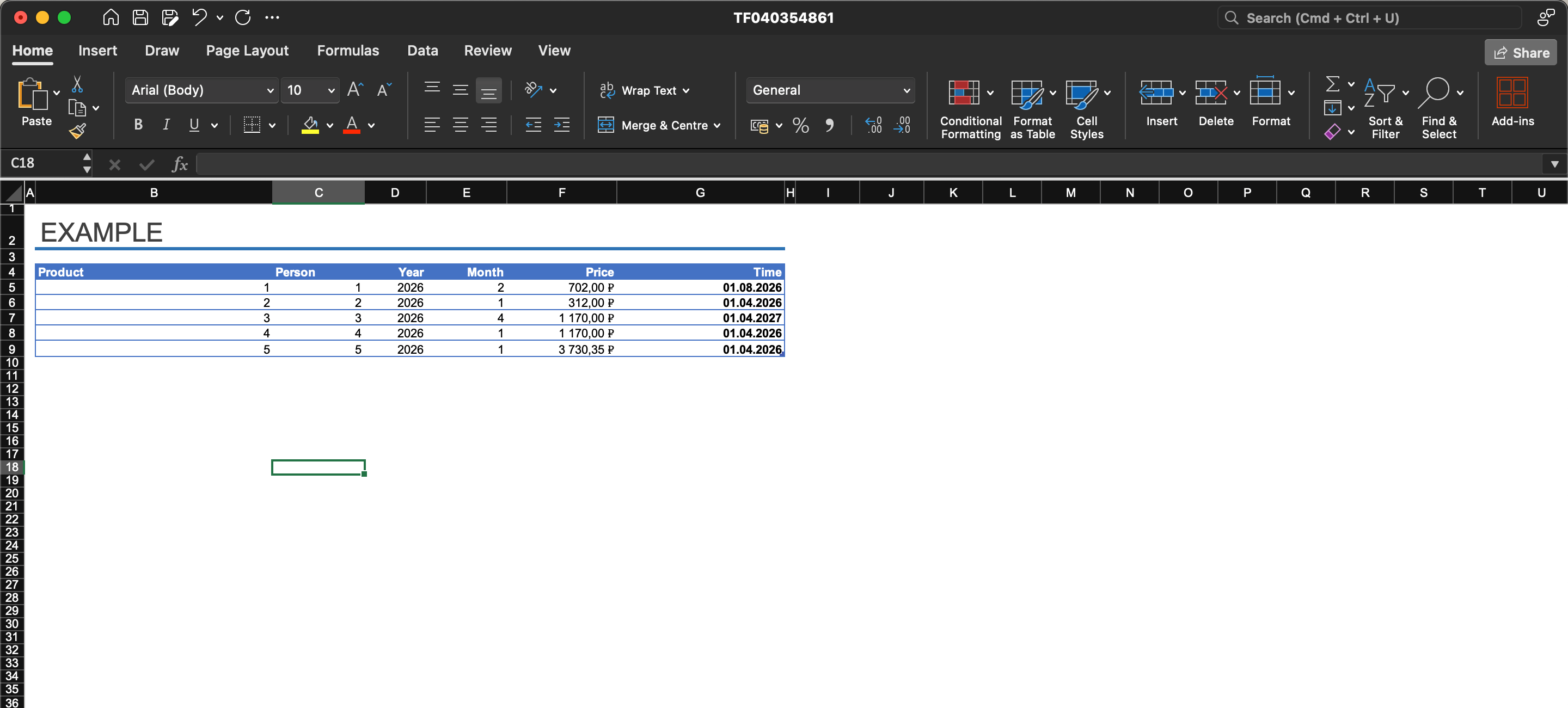
For a summary table to work correctly, it is important to fulfill several requirements:

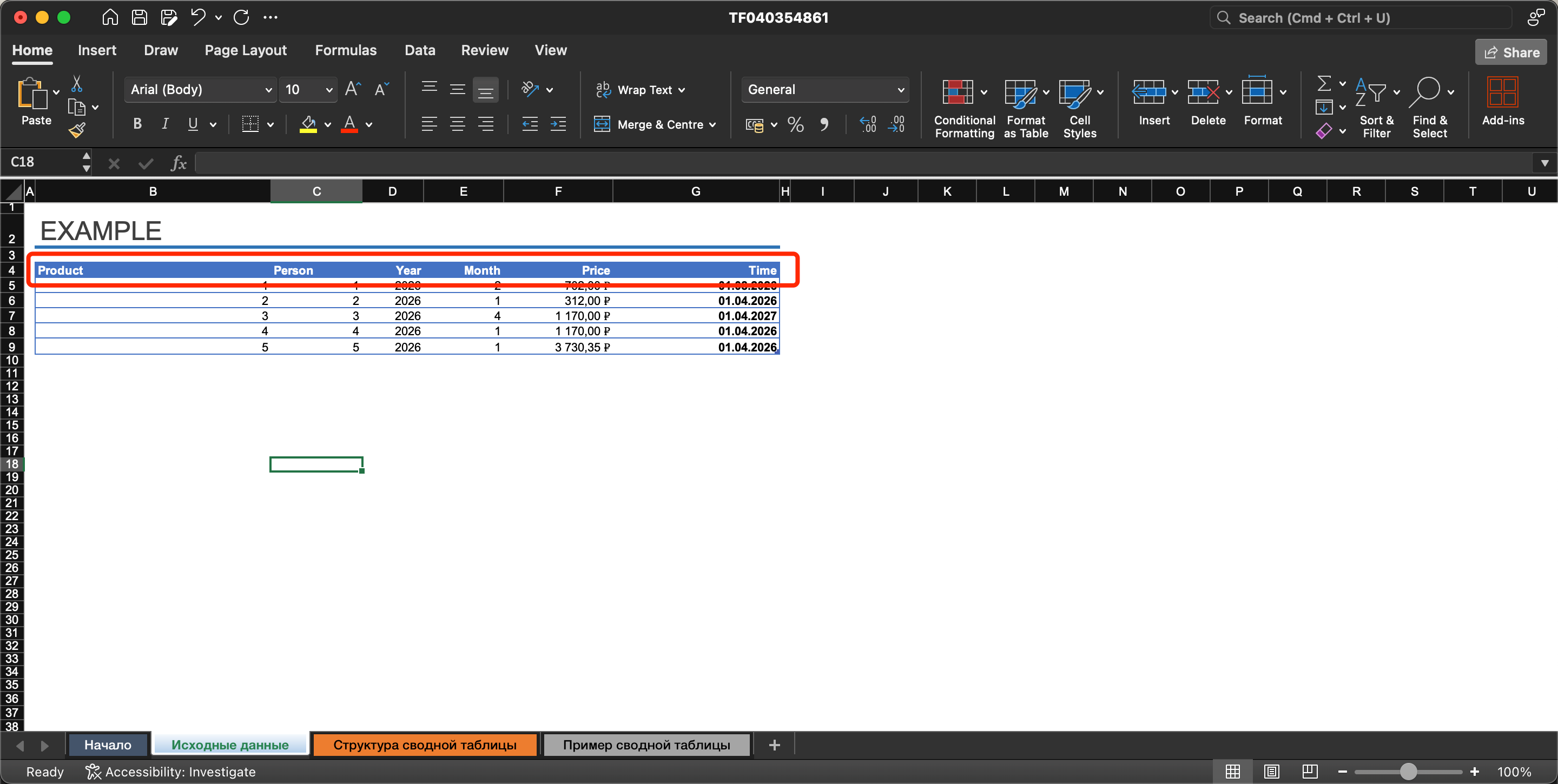
1. Each column must have its own heading.
   2. Each column requires one display format: number, date, and text.
   3. Cells and rows cannot be empty.

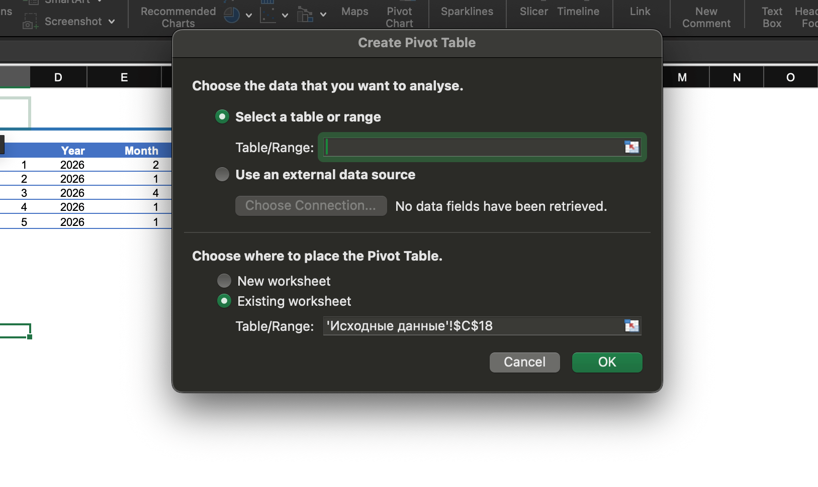
Next, select the Insert menu and find the Summary Table item.

This will display a dialog box where you must set two parameters:

• the range of the original table so that the summary table will get all the necessary information;
• the sheet to which the data will be moved for further processing.

We need to select the entire range together with the header and click on “New Sheet”, which will make it easier to move between the source values and the summary report. Click on “Ok”.

The program will generate a new sheet. You can immediately give it a name for comfortable work.

The left part of the sheet contains the area where the summary table is displayed after the adjustments have been made. The right side of the sheet contains the “Summary Table Fields” window, where these adjustments will be made. The next step is to figure out how to work with the panel.

Read also: Formulas and functions in Excel: How to use them to analyze data

Step 2: Customizing the Summary Table for the Result

At the top of the settings panel, you will find a block with a selection of valid summary table fields. These are borrowed from the column headers. In our case, these are: Product, Person, Year, Month, Price, time. There are four areas at the bottom of the panel: “Values”, ‘Columns’, ‘Rows’ and ‘Filters’. Each of them is intended for performing certain operations:

1. The Values section is responsible for performing calculations based on the table’s starting data and then transferring the results. In the standard mode, Excel performs data summation, but you can specify other actions, such as calculating the average, showing the minimum or maximum, multiplication. If the parameters are specified in numbers, Excel will find the sum of their values.
2. “Columns” and ‘Rows’ are for visual demonstration of fields in the table. If you specify “Rows”, the fields will be arranged line by line. If you select “Columns”, they are adapted to a columnar format.
3. “Filters”. This option is designed to filter the summary information in the summary table. Once it is built, the filters panel will be displayed separately. It has buttons to select the displayed data, as well as to hide it. For example, you can view sales of only one manager or for a specific period of time.

You can use two methods to customize the summary table:

1. Check the desired field. Excel will then decide where that value should be and automatically send it there.
   2. Select fields from the list and add them to the desired area using the manual method.

The first method is considered slightly unsuccessful. Excel rarely formats information in a way that makes it appear visually simple. As a result, the result looks uninformative.
As for the second method, personal customization for each report is allowed.
If we want only specific data to appear in the summary table, we should use filtering.

Step 3: Customizing Filters

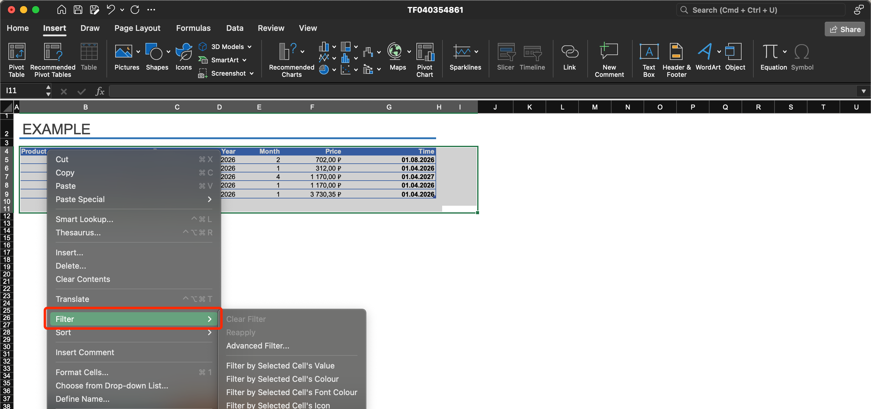
To more easily filter the data in our own summary table, we need to move the fields to the Filters menu. We can drag and drop all rows there.

Next, we can set filters by release date, for example by customizing the interface to show results for the second month.

Step 4: Update the data

If there is no data for any period in the summary table, such as the last month, but there is data in the source, the automatic transfer will not happen because the source range will change. In this case, you will need to change the starting values.

To do this, open the summary sheet, click the key in the Analyze Summary Sheet menu to change the source parameters. The key will send you to the source sheet, where you will need to set new range values. This will then automatically pull the information into the summary table. If there is a need to change parameters within the range, this too is done manually.

Thus, the ability to create summary tables will be a useful skill for all users working in Microsoft Office Excel. The capabilities of this office suite are enough to perform the most complex operations and calculations. And the summary tables perfectly systematize these data.